Analytical Tools

The Analytical Tools are only available in the Workspaces.

Accessing Analytical Tools

You can access the analytical tools by opening any new or existing workspace in the platform.

Getting to Know the Analytical Tools

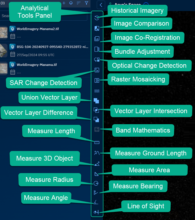
The Analytical Tools consists of many raster, vector, drawing, and measurement tools.

Historical Imagery

Use this tool to load and explore all available historical raster images for the area you're currently viewing on the map. Zoom into any region of interest, and the system will display a time-sequenced stack of imagery—from the oldest to the most recent. This enables you to visually track changes over time and analyze how the landscape or features have evolved based on available data.

Playing Historical Imagery

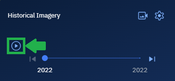
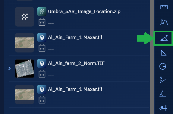
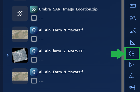
1. On the Analyst Tools, click the Historical Imagery icon to get started with using the tool.

   The Historical Imagery dialog box is displayed.

2. In the Historical Imagery dialog box, click the Play button to view all available historical raster images for the area you're currently viewing on the map.

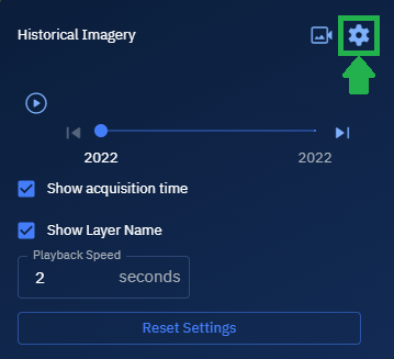
Editing the Play Settings

This settings enables you to display acquisition time and layer name while having better control of the historical imagery play.

3. In the Historical Imagery dialog box, click the Settings icon and do the following:
   • Select the Show Acquisition Time check-box to display imagery acquisition time on the play timeline.
   • Select the Show Layer Name check-box to display the layer name on the play timeline.
   • Type a number in the Playback Speed field to increase or decrease the playback speed in seconds.

Export the Image

This setting enables you to download image in PNG or JPEG format. You can also add acquisition date and time on the downloaded image. You can also design the text styling, background styling, and placement of the date and time label on the image.

4. In the Historical Imagery dialog box, click the Export icon.

5. Select PNG or JPEG as the image format that you want to download.

6. Select the Add acquisition date-time on image check-box, and then proceed to set up the text styling, background styling, and placement of the date and time label on the image.

7. Click the Download button to download the image to your local computer.

   

Image Comparison Tool

With the Image Comparison tool, you can visually compare two raster images side-by-side to identify spatial differences, detect visual changes, or confirm image alignment.

You can use this tool to quickly assess how a location has evolved between two points in time, compare different sensor outputs, or validate preprocessing accuracy. This tool is especially helpful when reviewing results from change detection or image correction workflows.

Prerequisites

Before using the Image Comparison tool, ensure the following:

• Two raster image layers are available in the Layers panel.
• Both images are georeferenced and aligned spatially for meaningful visual comparison.
• The images are in compatible formats and use a visible spectral band or RGB composite.

Use Cases

Use Case	Description
Change monitoring	Visually assess surface changes between two dates using side-by-side or swipe comparison.
Pre- and post-disaster review	Compare damage extent by switching between before-and-after imagery.
Sensor validation	Compare imagery from different satellites or sensors for consistency or calibration.
Workflow result validation	Confirm output of tools such as co-registration or change detection by visual inspection.
Feature tracking	Follow the growth, removal, or movement of land cover or man-made structures.

Configuring Parameters and Execute Job

To use the Image Comparison tool, do the following:

1. Go to the Analyst Tools panel, click the Image Comparison tool.

   

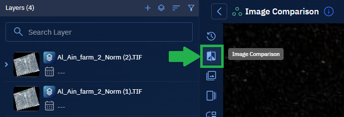
   The Image Comparison dialog box is displayed.

2. On the Image Comparison dialog box:

   • Select the First Image layer.

   • Select the Second Image layer to compare it with.

     

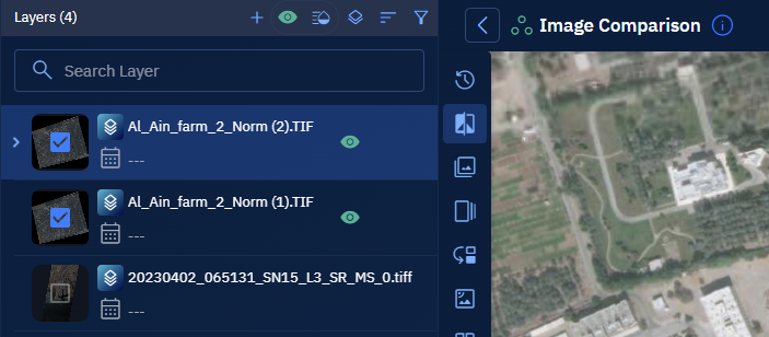
     A comparison slider is displayed on the screen.

Viewing and Validate the Results

3. Use the comparison slider to view and compare the two images.

   

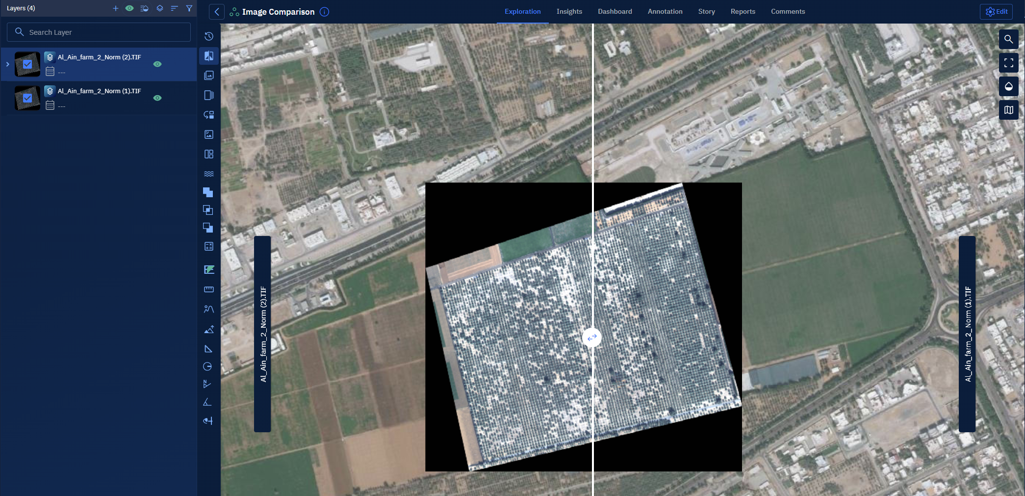
Image Co-Registration Tool

With the Image Co-Registration tool, you can align multiple raster images—captured from different times, sensors, or angles—so that they share the same spatial coordinate system. You can use this tool to ensure accurate pixel-to-pixel correspondence, enabling meaningful comparison, analysis, or fusion of imagery. This is especially useful when working with multi-temporal satellite data or integrating imagery from different sources.

Prerequisites

Before using the Image Co-Registration tool, ensure the following:

• At least two raster image layers are available in the Layers panel.
• Input images must have visible or identifiable features to match between them.
• All images must be in a known projection and contain georeferencing metadata.

Use Cases

Use Case	Description
Multi-temporal analysis	Align images from different dates to assess environmental or infrastructure change.
Sensor fusion	Overlay images from different satellites or cameras for comparative or blended analysis.
Preprocessing for change detection	Align imagery before applying optical or SAR change detection tools.
Image enhancement	Co-register higher-resolution and lower-resolution images for sharpening or detail preservation.
Accuracy improvement	Improve geolocation accuracy by correcting misalignments caused by acquisition differences.

Configuring Parameters and Execute Job

To use the Image Co-Registration tool, do the following:

1. Go to the Analyst Tools panel, click the Image Co-Registration tool.

   

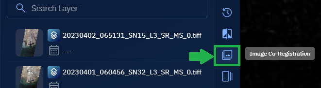
   The Image Co-Registration dialog box is displayed.

2. On the Image Co-Registration dialog box:

   • Select the Reference Image (the image to align to).
   • Select the Target Image (the image that will be shifted or warped to match the reference).
   • (Optional) Specify the tie points manually or allow the tool to auto-detect control points.
   • (Optional) Adjust transformation method if available (e.g., affine, polynomial, or spline).

3. Click the Apply button to align the target image with the reference image.
   A new co-registered image layer is generated and added to the workspace.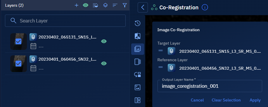

   

Monitoring Processing Pipeline

4. Click the Data module, select the Analytics sub-module, and then view the job progress in the In-Progress/Completed tab.

   
   

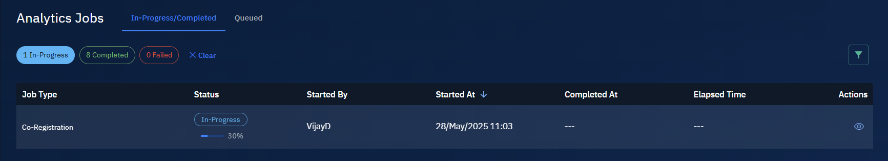
   Once the job is successfully processed, it will be displayed in the Workspace.

note

Click the Eye icon to view details of the job.

Viewing and Validate the Results

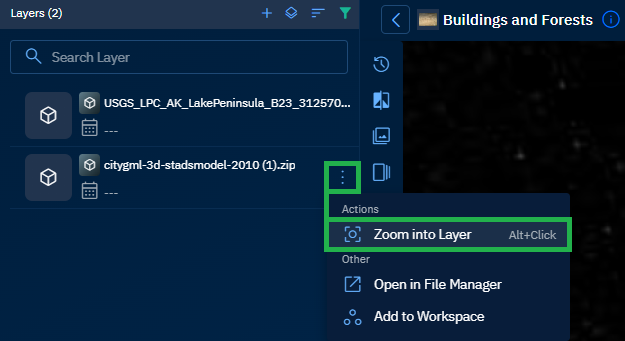
5. In the Workspace, select the output layer, click the vertical three-dots menu, and then click Zoom into Layer to review and interpret the changes.

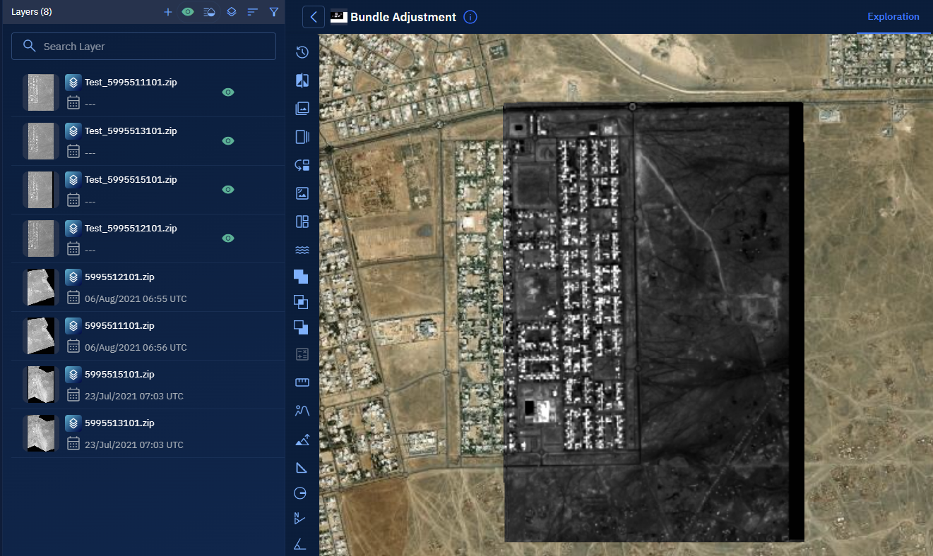
Bundle Adjustment Tool

With the Bundle Adjustment tool, you can optimize both 3D point positions and camera parameters across multiple overlapping images. You can use this tool to improve the accuracy of photogrammetric reconstructions by minimizing projection errors between observed and calculated image points.

This is especially useful when working with drone imagery, aerial photographs, or multi-angle satellite scenes.

Prerequisites

Before using the Bundle Adjustment tool, ensure the following:

• Input images must be overlapping images with associated camera models or metadata
• Input images must be georeferenced or contain orientation data (e.g., GPS/IMU)
• Input images must be from a single vendor only. In the current release, only Airbus is supported.
• Input images must be multispectral images

Use Cases

Use Case	Description
Aerial mapping correction	Refine the alignment of overlapping drone or aerial images to improve 3D model accuracy.
3D point cloud refinement	Enhance the precision of 3D scene reconstruction from multiple image sources.
Orthophoto generation	Prepare images for orthorectification by correcting internal camera distortions.
Survey-grade accuracy	Achieve high positional accuracy for applications such as cadastral mapping or engineering surveys.

Configuring Parameters and Execute Job

To use the Bundle Adjustment tool, do the following:

1. Go to the Analyst Tools panel, click the Bundle Adjustment tool.

   

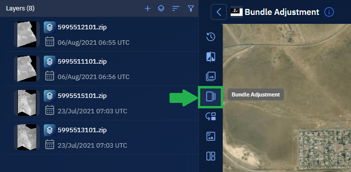
   The Bundle Adjustment dialog box is displayed.

2. On the Bundle Adjustment dialog box, do the following:

   • Click the Select Vendor drop-down list and select a vendor
   • Draw an Area of Interest (AOI) with square tool
   • Select a minimum of two overlapping images

3. Click the Apply button to run the bundle adjustment process.
   The tool will optimize image orientation and 3D point locations across the dataset.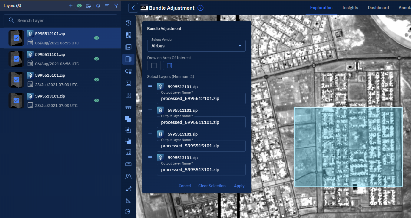

   

Monitoring Processing Pipeline

4. Click the Data module, select the Analytics sub-module, and then view the job progress in the In-Progress/Completed tab.

   
   

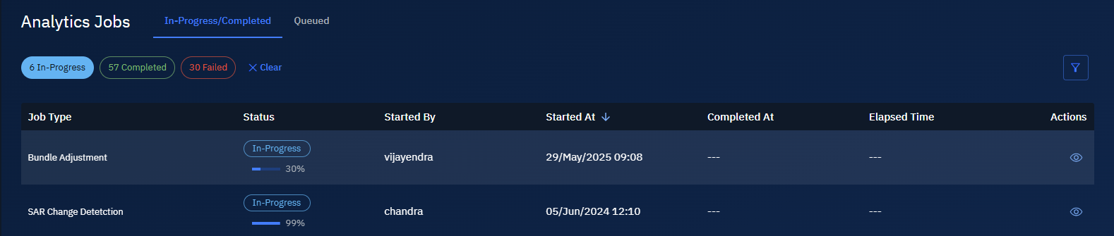
   Once the job is successfully processed, it will be displayed in the Workspace.

note

Click the Eye icon to view details of the job.

Viewing and Validate the Results

5. In the Workspace, select the output layer, click the vertical three-dots menu, and then click Zoom into Layer to review and interpret the changes.

   

Optical Change Detection Tool

With the Optical Change Detection tool, you can analyze optical imagery taken at two different time points to identify changes on the Earth’s surface. By comparing images from visible and near-infrared bands, you can detect variations in land use, vegetation, infrastructure, or natural events.

You can use this tool to uncover surface-level changes using data from satellites or aerial sensors equipped with optical cameras.

Prerequisites

Before using the Optical Change Detection tool, ensure the following:

• Two optical image layers, captured at different time points, are available in the Layers panel.
• Input layers must be georeferenced and aligned spatially.
• Both images must be from the same sensor type or have consistent spectral bands.

Use Cases

Use Case	Description
Urban expansion monitoring	Detect construction, road development, or city boundary growth.
Vegetation and crop tracking	Identify deforestation, seasonal crop cycles, or degradation.
Disaster assessment	Analyze damage caused by fires, floods, or earthquakes over time.
Environmental monitoring	Track wetland shrinkage, coastal erosion, or habitat changes.
Land use classification	Compare classification results from different dates to map transition zones.

Configuring Parameters and Execute Job

To use the Optical Change Detection tool, do the following:

1. Go to the Analyst Tools panel, click the Optical Change Detection tool.

   

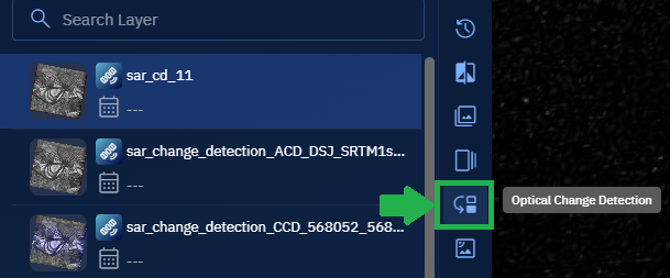
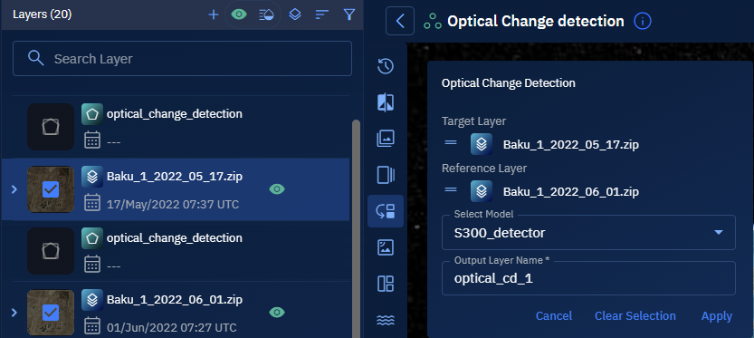
   The Optical Change Detection dialog box is displayed.

2. On the Optical Change Detection dialog box:

   • Select the Target Image (newer image or more recent acquisition).
   • Select the Reference Image (older image or baseline comparison).
   • Draw an Area of Interest (AOI) using a rectangle or polygon, or select from the AOI Library, or paste the WKT coordinates.

3. Click the Apply button to generate a change detection output based on spectral comparison of both images.

   

Monitoring Processing Pipeline

4. Click the Data module, select the Analytics sub-module, and then view the job progress in the In-Progress/Completed tab.

   
   

   Once the job is successfully processed, it will be displayed in the Workspace.

note

Click the Eye icon to view details of the job.

Viewing and Validate the Results

5. In the Workspace, select the output layer, click the vertical three-dots menu, and then click Zoom into Layer to review and interpret the changes.

   

SAR Change Detection Tool

With the SAR Change Detection tool, you can compare two SAR images taken at different times to detect and analyze changes.

You can use this tool to monitor activity and assess change over time using radar-based imagery—regardless of weather or daylight conditions. Some of the typical changes you can detect include shifts in vegetation, urban development, flood damage, and so on.

Prerequisites

Before using the SAR Change Detection tool, ensure the following:

For Amplitude Change Detection:

• Must select a SAR Layer
• Same satellite name
• The recommended product level to use is GRD (Ground Range Detected). GRD products provide detected (magnitude-only) images in ground-range coordinates, making them suitable for analyzing changes in amplitude.
• Same orbit direction
• Same look side
• Must overlap by 90%

For SLC Coherence Change Direction:

• Must select a SAR Layer
• Same satellite name
• The recommended product level to use is SLC (Single Look Complex). SLC products preserve the raw complex signal (amplitude and phase) in slant-range geometry, which is more suitable for interferometry-based change detection
• Same orbit direction
• Same look side
• Incidence angle should me similar
• Should overlap by 90%

Use Cases

Use Case	Description
Urban change detection	Monitoring infrastructure expansion or development between two time periods.
Flood or disaster analysis	Identify areas affected by flooding, landslides, or other surface disruptions.
Vegetation tracking	Detect seasonal or human-driven changes in vegetation cover.
Conflict zone monitoring	Observe structural or terrain shifts in areas of interest.
Coherence analysis	Evaluate structural stability or surface changes using SLC Coherence.

Configuring Parameters and Execute Job

To use the SAR Change Detection tool, do the following:

1. Go to the Analyst Tools panel, and click the SAR Change Detection tool.

   

   The SAR Change Detection dialog box is displayed.

2. On the dialog box, configure the following options:
   

Field	Description
Select Workflow	Choose the change detection method: Amplitude Change Detection compares brightness (intensity) between two SAR images. SLC Coherence Change Detection compares phase similarity to detect fine surface changes. 💡 Use Amplitude for floods or land-cover change; use SLC Coherence for construction or terrain stability.
Target Layer	Select the later-date SAR image. This is the layer where changes are expected.
Reference Layer	Select the earlier-date SAR image to compare against.
Advanced Parameters	Select one of the following options.
Digital Elevation Model (DEM)	Choose the elevation model for terrain correction: Auto SRTM 1Sec HGT SRTM 3Sec Copernicus 30m Global DEM Copernicus 90m Global DEM 💡 Use higher-resolution DEMs like Copernicus 30m for mountainous areas.
Polarization	Select matching polarization for both images: VV VH HH HV 💡 Use VV for general land cover; VH for vegetation.
Geometric Correction	Choose how spatial distortion is corrected: Auto Terrain Correction Ellipsoid Correction 💡 Use Terrain Correction for precise surface mapping; Ellipsoid for flat regions.
N Looks	Type or select a number (e.g., 1–5) to adjust speckle filtering. 💡 Higher values (e.g., 3–5) reduce noise; lower values retain detail.
Mask UAE Sea	Choose whether to exclude sea/water bodies: Activate Deactivate 💡 Activate masking for land-based analysis only.

3. Click the Apply button to run the SAR change detection.

   

   The system processes both layers and generates a change map.
   

Monitoring Processing Pipeline

4. Click the Data module, select the Analytics sub-module, and then view the job progress in the In-Progress/Completed tab.

   
   

   Once the job is successfully processed, it will be displayed in the Workspace.

NOTE: Click the Eye icon to view details of the job.

Viewing and Validate the Results

5. In the Workspace, select the output layer, click the vertical three-dots menu, and then click Zoom into Layer to review and interpret the changes.

   

Raster Mosaicking Tool

The Raster Mosaicking tool allows you to combine multiple raster datasets—typically adjacent or overlapping tiles—into a single, continuous raster image. The input rasters may include satellite imagery, aerial photographs, elevation data, or other grid-based datasets. This process aligns, blends, and harmonizes the pixel values at the seams to create a seamless visual or analytical layer across a larger area.

Prerequisites

Before using the Raster Mosaicking tool, ensure the following:

• Only layers with 3 bands (RGB) are supported in the current release. The current release does not support mosaicking layers with band mismatches.
• Only .tif image format is supported in the current release
• A minimum of two and a maximum of four images can be combined together
• Input layers must have the same number of spectral bands. The current release does not support mosaicking layers with band mismatches.
• Spatial resolution difference between input layers must be within 20 percent to maintain quality and alignment.

Use Cases

Use Case	Description
Merging image tiles	Combines adjacent satellite or aerial image tiles into a single, continuous regional view.
Composite raster generation	Creates unified elevation, NDVI, or other thematic rasters by merging multiple segments.
Preprocessing for analysis	Prepares consistent raster layers for downstream tasks such as classification or modeling.
Seam removal	Eliminates visible seams or gaps between overlapping or neighboring raster tiles.

Configuring raster mosaicking parameters

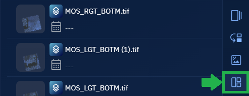
1. Go to the Analyst Tools panel, click the Raster Mosaicking tool.

   

   The Raster Mosaicking dialog box is displayed.

2. Select Layer 1 and Layer 2 from the Layers panel and view the selections on the Raster Mosaicking dialog box.

   

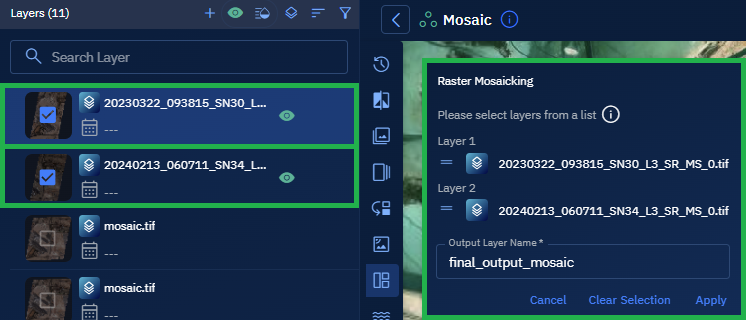
3. Type a name for the output file in the Output Layer Name field. For example, final_output_mosaic

4. Click Apply to start the raster mosaicking process.

   A confirmation message will be displayed on the screen.

System Executes and Publishes the Mosaicked Output

After you click the Apply button, the mosaicking job is submitted to the platform’s backend for automated processing.

• The job is routed to the Analytics sub-module, where it is queued and executed. Only roles with appropriate permissions can access the Analytics sub-module.
• Once processing is complete, the output is passed to the inference engine, which validates and finalizes the result.
• Upon successful validation, the final mosaicked image is automatically published to the Layers section in your Workspace.

This system-driven step includes:

• Georeferencing alignment
• Operator-based pixel processing
• Quality assurance and metadata checks

Note: This entire step is fully automated.
No user input or monitoring is required.

For more details, see the Data > Jobs > Analytics sub-module chapter.

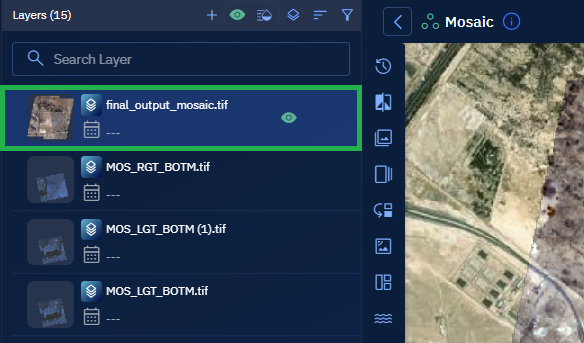
Viewing and Confirm the Mosaicked Output

5. Go to the Layers section in your workspace, locate the newly generated mosaicked image, and click the layer name to view it on the map.

Visually inspect the layer to confirm that:

• The tile boundaries have been blended correctly.
• Color maps appear as expected (if applied).
• No visible seams or alignment issues remain.

Optional:
If you want to download a local copy of the output:

1. Select the mosaicked image in the Layers panel. The Contextual Panel slides out.
2. Go to the Properties tab in the contextual image panel.
3. Click the Download icon (down arrow) to save the file to your computer.

Vector Layer Union Tool

With the Vector Layer Union tool, you can combine vector features from two separate files into a single, unified output layer. You can merge overlapping features into one, while preserving non-overlapping features as individual entries in the same file.

This helps you build a complete dataset that represents both shared and unique geometries across sources—whether you're working with points, lines, or polygons.

Prerequisites

Before using the Vector Layer Union tool, ensure the following:

• Two input layers must be available in the Layers panel.

Use Cases

Use Case	Description
Unified spatial data	Combine multiple vector layers into one consolidated layer for visualization or analysis.
Feature merging	Merge overlapping geometries into single features to eliminate redundancy.
Spatial completeness	Ensure no spatial data is excluded, even when input features don’t intersect.
Layer consolidation	Reduce multiple sources into one vector file for easier management and analysis.

Using Vector Layer Union Tool

In this section, you will learn how to use the Vector Layer Union tool.

To use the Vector Layer Union tool, do the following:

1. Go to the Analyst Tools panel, click the Vector Layer Union tool.

   

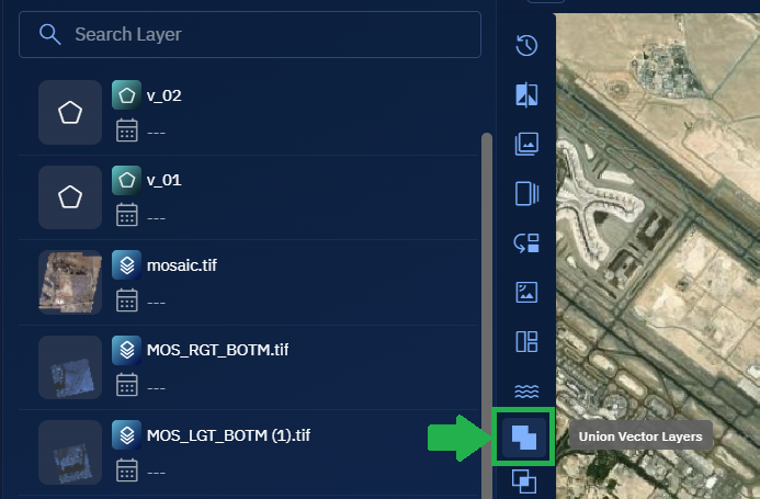
   The Vector Layer Union dialog box is displayed.

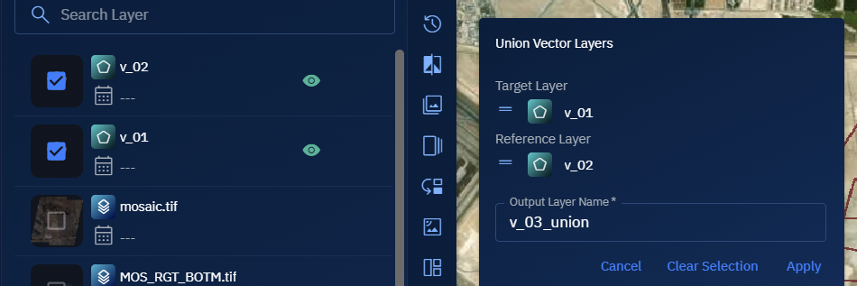
2. On the Vector Layer Union dialog box:

   • Select the First Layer.
   • Select the Second Layer to union with the first.

3. Click the Apply button to create a single output layer that merges overlapping features into one and retains non-overlapping features as separate entries.

   

4. Select the output layer, click the vertical three-dots menu, and then click the Zoom into Layer option. Proceed to review all the combined features on the map.

   

Vector Layer Intersection Tool

The Vector Layer Intersection tool is used to extract spatial features that are common to two vector layers. It performs a geometric overlay operation to identify areas or features that exist in both layers, and outputs a new vector layer containing only those intersecting parts.

This operation is applicable to vector data types such as points, lines, and polygons, and is widely used in spatial analysis workflows to detect overlaps, shared boundaries, or jointly occupied spaces.

Prerequisites

Before using the Vector Layer Intersection tool, ensure the following:

• Both input layers must be vector layers (point, line, or polygon).
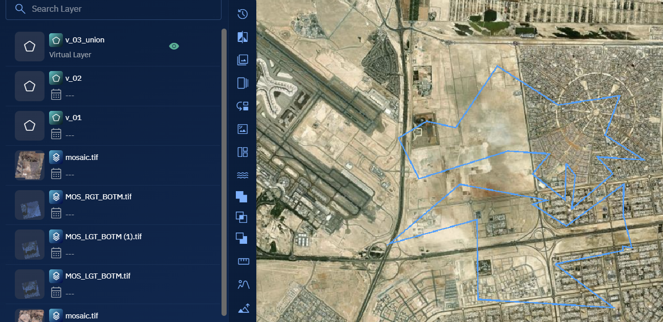
• The input layers are available in the Layers panel.
• The geometry types of the input layers are compatible for intersection.
• Both layers must be correctly georeferenced and aligned spatially.

Use Cases

Use Case	Description
Overlap analysis	Identify areas where two zones or jurisdictions share common ground.
Shared infrastructure	Find where road networks intersect with pipelines, or where habitats overlap with utility lines.
Land use constraints	Determine where proposed development areas intersect with protected zones or hazard zones.
Spatial querying	Generate a new dataset containing only features that are spatially common to both input layers.

Using Vector Layer Intersection Tool

In this section, you will learn how to use the Vector Layer Intersection tool.

To use the Vector Layer Intersection tool, do the following:

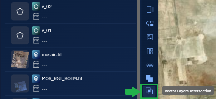
1. Go to the Analyst Tools panel, click the Vector Layer Intersection tool.

   

   The Vector Layer Intersection dialog box is displayed.

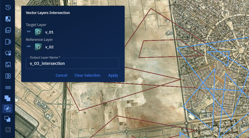
2. On the Vector Layer Intersection dialog box:

   • Select the First Vector Layer (v_01).
   • Select the Second Vector Layer (v_02) to intersect with the first layer.
   

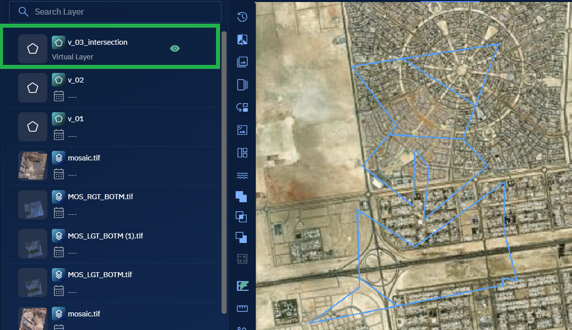
3. Click the Apply button to generate a new layer containing only features that exist in both input layers.

   The resulting output layer is automatically added to the Layers panel. This layer contains only those spatial features where the two selected layers overlap.

4. Select the output layer, click the vertical three-dots menu, and then click the Zoom into Layer option. Proceed to view the features.

   

Vector Layers Difference Tool

The Vector Layers Difference tool is used to identify unique features in the target vector layer that do not exist in the reference vector layer.

You can use this tool to perform a geometric subtraction operation, resulting in a new layer that contains only the features unique to the target.

This tool supports vector data types such as points, lines, and polygons, and is commonly used in spatial analysis to highlight areas of change, exclusion, or discrepancy between datasets.

Prerequisites

Before using the Vector Layers Difference tool, ensure the following:

• Input layers are of the same geometry type (for example, both layers must contain polygons, lines, or points).

Use Cases

Use Case	Description
Change detection	Identify new constructions, expansions, or land use changes by comparing updated survey data with baseline layers.
Data validation	Highlight discrepancies between a planned dataset and what actually exists on the ground.
Spatial cleanup	Remove overlapping or duplicate geometries from the target dataset based on reference standards.
Regulatory compliance	Ensure a proposed boundary or plan does not intrude into restricted zones defined in the reference layer.

Using Vector Layers Difference Tool

In this section, you will learn how to use the Vector Layers Difference tool.

Configuring Parameters and Execute Job

To use the Vector Layers Difference tool, do the following:

1. Go to the Analyst Tools panel, click the Vector Layers Difference tool.

   

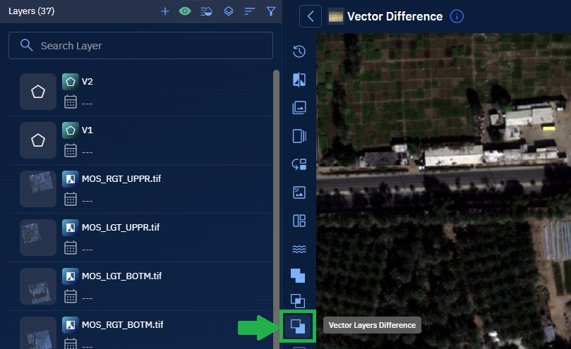
   The Vector Layers Difference dialog box is displayed.

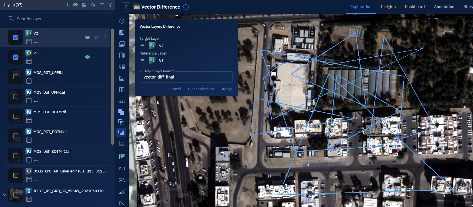
2. On the Vector Layers Difference dialog box:

   • Select the Target Layer (the layer from which features will be subtracted).
   • Select the Reference Layer (the layer whose features will be used to perform the subtraction).

3. Click the Apply button to run the difference operation.

   A new output layer is generated containing features that exist in the target layer but not in the reference layer. This output is automatically added to the Layers panel for visualization and further analysis.

   

Monitoring Processing Pipeline

4. Click the Data module, select the Analytics sub-module, and then view the job progress in the In-Progress/Completed tab.

   

   Once the job is successfully processed, it will be displayed in the Workspace.

NOTE: Click the Eye icon to view details of the job.

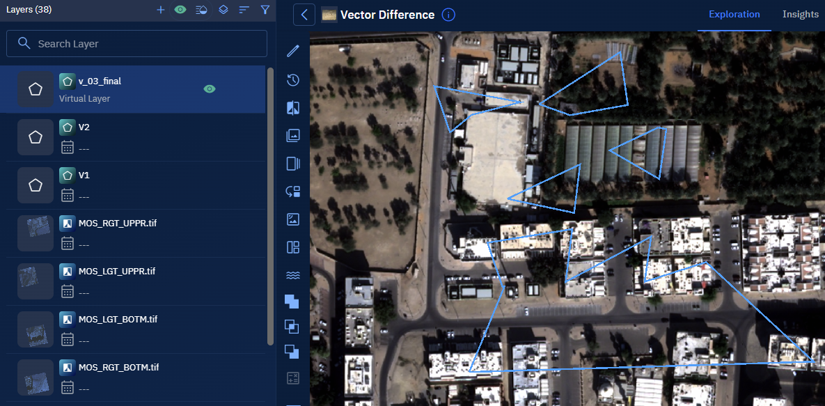
Viewing and Validate the Results

5. Select the virtual output layer, click the vertical three-dots menu, and then click the Zoom into Layer option. Proceed to view the features.

   

Band Mathematics Tool

Use the Band Mathematics tool to derive new raster outputs by applying mathematical expressions to individual bands in a multi-band raster layer. You can create custom indices (like NDVI), enhance spectral features, or isolate phenomena by performing pixel-wise operations across bands.

Prerequisites

Before using the Band Mathematics tool, ensure the following:

• The raster layer includes clearly defined band metadata.
• You must know the band names or indexes to reference in the expression (e.g., B4, B8).
• You must be familiar with basic arithmetic operations and their application to raster data.

Use Cases

Use Case	Description
Deriving vegetation indices	Calculate NDVI or similar metrics to assess vegetation health or cover density.
Creating custom raster layers	Combine specific bands to highlight moisture, heat, or urban change patterns.
Enhancing visual contrast or spectral features	Use formulas to emphasize land, water, or built-up areas.
Masking or filtering data conditionally	Apply logical conditions to exclude unwanted pixels or highlight anomalies.

---

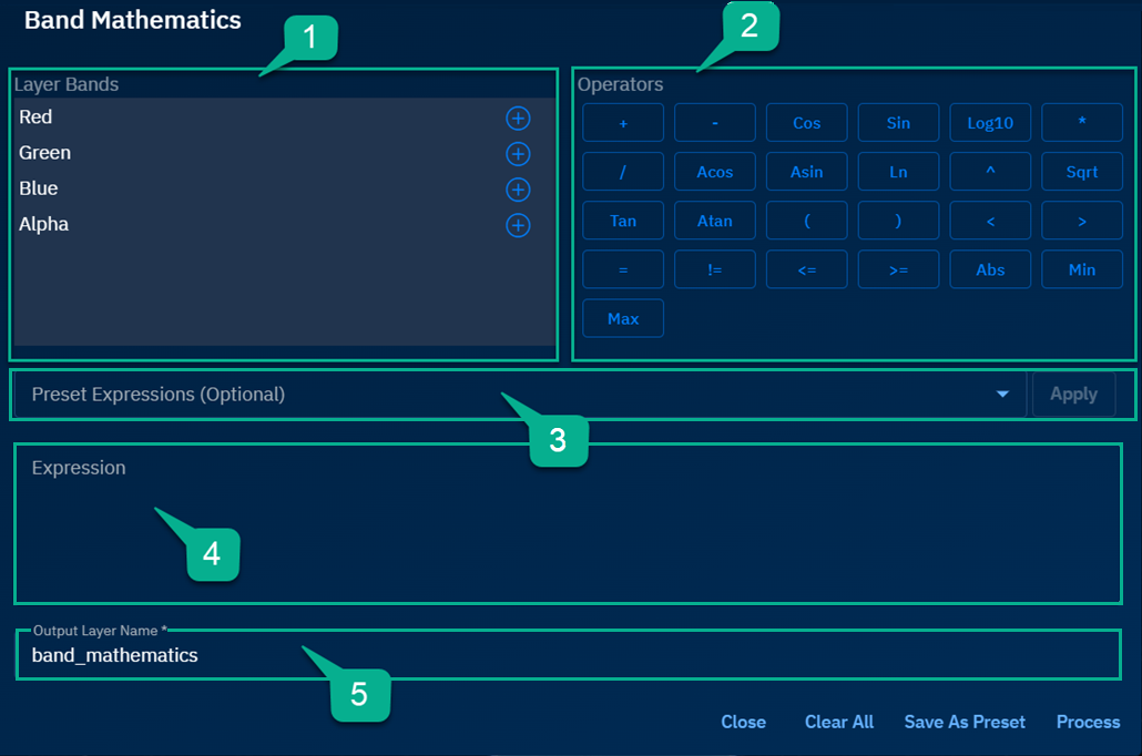
Band Mathematics Interface

No.	Field	Description	Examples
1	Layer Bands	Represents individual bands from a multi-band raster dataset. Each band captures different spectral information such as Red, Green, Blue, or NIR.	B1 for Blue, B4 for Red, B8 for NIR
2	Operators	A set of mathematical and logical expressions used to create raster formulas. Includes arithmetic, comparison, and trigonometric functions. See the Examples of Operators chapter for more information.	+, -, /, *, log(), sqrt(), sin(), ==, >
3	Preset Expressions	Built-in expressions provided for common raster calculations. When selected, these auto-fill the expression field with a formula that the user can modify. See the Descriptions of Preset Expressions chapter for more information.	NDVI = (B8 - B4) / (B8 + B4) SAVI = ((B8 - B4) / (B8 + B4 + L)) * (1 + L)
4	Expression	The custom mathematical formula you define using available bands and operators. This is the core input that drives the band math calculation.	(B8 - B4) / (B8 + B4) sqrt(B11) * log(B4 + 1)
5	Output Layer Name	The name for the output raster layer that will be generated after executing the band math expression.	NDVI_March2024 Vegetation_Index_Output

Examples of Operators

This section presents mathematical and logical expressions examples for arithmetic, comparison, and trigonometric functions.

| Operator Type | Operator / Function | Description | Example | | ------------------- | ------------------------------- | --------------------------------------------------------- | ------------------------------------------------------- | ----- | --------- | | Arithmetic | + (Addition) | Adds values from two rasters | raster1 + raster2 adds values pixel-wise | | | - (Subtraction) | Subtracts a constant or raster from another raster | raster1 - 5 subtracts 5 from every pixel in raster1 | | | * (Multiplication) | Multiplies each pixel value by a constant or raster | raster * 2 multiplies every value in raster by 2 | | | / (Division) | Divides the values of one raster by another | raster1 / raster2 divides raster1 values by raster2 | | Comparison | = (Equal to) | Checks if values in two rasters are equal | raster1 = raster2 returns True where values match | | | != (Not equal to) | Checks if values are not equal | raster1 != raster2 returns True where values differ | | | < (Less than) | Checks if raster values are less than a threshold | raster1 < 10 returns True for pixels < 10 | | | <= (Less than or equal to) | Checks if raster values are less than or equal to another | raster1 <= raster2 returns True where condition holds | | | > (Greater than) | Checks if raster values are greater than a threshold | raster1 > 5 returns True for pixels > 5 | | | >= (Greater than or equal to) | Checks if raster values are ≥ a threshold | raster1 >= 0 returns True where values ≥ 0 | | Mathematical | sqrt(x) | Returns the square root of each raster value | sqrt(raster1) returns sqrt of each pixel | | | log(x) | Returns the natural logarithm of each raster value | log(raster1) returns ln of each pixel | | | ln(x) | Computes the natural logarithm (base e) of x | ln(raster1) returns ln of each pixel | | | abs(x) | Returns the absolute value of each raster value | abs(raster1) returns | value | per pixel | | Trigonometric | sin(x) | Returns the sine of an angle (in radians) | sin(raster1) returns sine of pixel values | | | cos(x) | Returns the cosine of an angle (in radians) | cos(raster1) returns cosine of pixel values | | | tan(x) | Returns the tangent of an angle (in radians) | tan(raster1) returns tangent of pixel values | | | Asin(x) | Returns the arcsine of x (in radians) | Asin(raster1) returns arcsine of values | | | Acos(x) | Returns the arccosine of x (in radians) | Acos(raster1) returns arccosine of values | | | Atan(x) | Returns the arctangent of x (in radians) | Atan(raster1) returns arctangent of values | | Other Functions | ^ (Exponentiation) | Raises a value to a power | raster1 ^ 2 squares each pixel | | | ( (Left parenthesis) | Groups expressions and controls order of operations | sqrt((raster1 + raster2) * 2) | | | ) (Right parenthesis) | Closes grouped expressions for order control | log((raster1 + 1)) |

Descriptions of Preset Expressions

Preset Expression Name	Formula	Purpose	How to Use
Brightness Index	sqrt(("[R]"^2+"[G]"^2+"[B]"^2)/3)	Measures surface brightness in arid regions	Use in areas with exposed soil to estimate surface brightness.
Soil Color Index	("[R]"-"[G]")/("[R]"+"[G]")	Highlights bare soil characteristics	Apply on bare soil zones to distinguish different soil colors.
Green Leaf Index	(2*"[G]"-"[R]"-"[B]")/(2*"[G]"+"[R]"+"[B]")	Emphasizes green vegetation, suppresses soil	Best used to enhance visualization of healthy green vegetation.
Primary Colors Hue Index	(2*"[R]"-"[G]"-"[B]")/("[G]"-"[B]")	Estimates hue from primary colors	Apply to RGB composites for color hue classification.
Normalized Green Red Difference Index	("[G]"-"[R]")/("[G]"+"[R]")	Vegetation index alternative to NDVI	Use when NIR is unavailable, especially in basic RGB imagery.
Spectral Slope Saturation Index	("[R]"-"[B]")/("[R]"+"[B]")	Measures spectral slope and vegetation types	Apply to distinguish vegetation from water or other surfaces.
Visible Atmospherically Resistant Index	("[G]"-"[R]")/("[G]"+"[R]"-"[B]")	Vegetation detection using visible bands	Best for visible-spectrum-only vegetation analysis.
Overall Hue Index	atan(2*("[B]"-"[G]"-"[R]")/30.5*("[G]"-"[R]"))	Abstract hue metric	Use for analyzing hue variations in RGB imagery.
Blue Green Pigment Index	"[B]"/"[G]"	Differentiates water and green pigments	Apply in water and plant separation tasks.
Plant Senescence Reflectance Index	("[R]"-"[G]")/("[RE]")	Detects plant senescence and pigment loss	Use to detect aging or dying vegetation during crop monitoring.
Normalized Difference Vegetation Index	("[NIR]"-"[R]")/("[NIR]"+"[R]")	Measures green vegetation health	Standard vegetation health monitoring index.
Green NDVI (GNDVI)	("[NIR]"-"[G]")/("[NIR]"+"[G]")	Sensitive to chlorophyll content	Use for precision chlorophyll mapping in agricultural fields.
Ratio Vegetation Index	"[NIR]"/"[R]"	Simple vegetation health ratio	Apply for quick assessment of vegetation density.
Normalized Difference Red Edge Index	("[NIR]"-"[RE]")/("[NIR]"+"[RE]")	Detects mature vegetation chlorophyll	Use in crops to detect stress earlier than NDVI.
Triangular Vegetation Index	0.5*(120*("[NIR]"-"[G]")-200*("[R]"-"[G]"))	Detects green biomass and canopy structure	Apply in dense vegetation areas to detect canopy structure.
Chlorophyll Vegetation Index	("[NIR]"*"[R]")/("[G]"^2)	Highlights chlorophyll abundance	Use to map chlorophyll concentration across regions.
Enhanced Vegetation Index (EVI)	2.5*("[NIR]"-"[R]")/("[NIR]"+6*"[R]"-7.5*"[B]"+1)	Improves sensitivity in high biomass and reduces haze	Apply where atmospheric correction is critical in high biomass.
Chlorophyll Index - Green	("[NIR]"/"[G]")-1	Estimates leaf chlorophyll using green band	Best for green vegetation detection using simpler sensors.
Chlorophyll Index - Red Edge	("[NIR]"/"[RE]")-1	Detects subtle chlorophyll changes	Apply for detailed crop health assessment.
Difference Vegetation Index	"[NIR]"-"[RE]"	Basic vegetation index for health and stress analysis	Use for direct NIR-red difference vegetation evaluation.

Starting a Band Mathematics Job

In this section, you will learn how to use the Band Mathematics tool.

You can use band mathematics in two ways:

• Use the preset expressions
• Create and use you own custom expressions

Using Preset Expressions

The system provides predefined expressions for common raster calculations. To use a preset, select it from the list, assign the required bands, and the expression is applied automatically.

To use the present expressions, do the following:

1. Click the Preset Expressions drop-down list, select a preset expression. For example, Green Normalized Difference Vegetation.

   

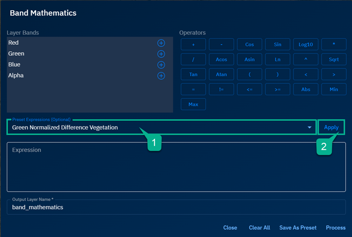
2. Click the Apply button to assign bands and generate the expression.

   A dialog box for the preset expression is displayed.

3. In the dialog box, view the formula of the expression and the bands needed for the formula.

   

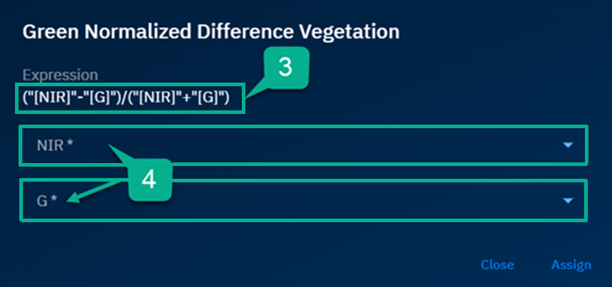
4. Verify the bands needed for the formula.

5. Select the bands needed for the formula and then click the Assign button to generate the expression using the selected bands.

   

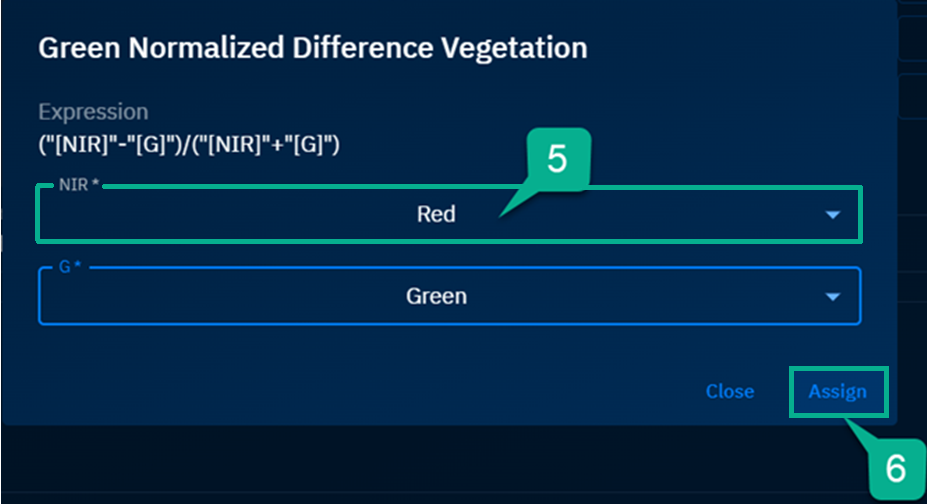
6. Click the Assign button to generate the expression using the selected bands.

Creating custom expressions

Users can create custom expressions using layer bands and supported operators. They can also modify expressions generated from presets and use them for raster calculations.

To create custom expressions, do the following:

1. Open a workspace and then select an image to run band mathematics.

2. In the Analyst Tools, select the Band Mathematics icon to get started. The Band Mathematics dialog box is displayed.

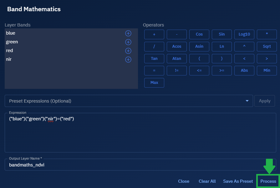
3. In the Band Mathematics dialog box, click the Expression field to start building your custom expression.

4. In the Output Layer Name, type an appropriate name for the output layer.

5. Click the Process button to start the band mathematics analytical job.

   

Reviewing the Output

You can review the final output within the workspace.

To review the output, do the following:

1. Navigate to the Layers section in your workspace.

2. Locate the newly generated raster layer by the name you provided.

3. Click the output layer to visualize it on the map.

4. To inspect the result:

   • Hover over or click pixels (if supported) to review output values.
   • Confirm that the expression was applied correctly and the data represents your intent.

5. Optionally, click the vertical three-dots menu next to the output layer and select Zoom into Layer to focus on the processed region.

note

You can download the final raster by selecting the layer, opening the Properties tab, and clicking the Download icon.

Measure Length Tool

The Measure Length tool is used to calculate the straight-line distance between two points on the map. This measurement represents the shortest linear path over a flat surface, without accounting for terrain elevation.

This tool is ideal for quick, planar measurements between two locations.

Prerequisites

• Open a workspace with any visible map layer.

Use Cases

The Measure Length tool is useful in scenarios where accurate, straight-line distances are required:

Use Case	Description
Distance Estimation	Quickly calculate direct distances between two geographic points.
Site Planning	Measure spacing between infrastructure elements like roads, fences, or plots.
Navigation Checks	Validate the shortest path between two fixed locations.
Construction Layout	Plan straight sections of pipelines, roads, or utility lines.

Using Measure Length Tool

In this section, you will learn how to use the Measure Length tool.

To use the Measure Length tool, do this:

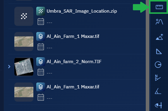
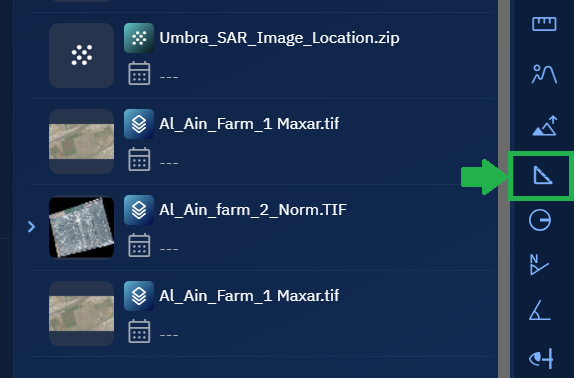
1. Go to the Analyst Tools panel, click Measure Length tool.

   

   The Measurements dialog box is displayed.

2. On the Measurements dialog box, click the Measure Units drop-down list to select one of the following units of measurement:

   • Meters
   • Kilometers
   • Feet
   • Miles
   • Nautical Miles

note

This unit determines how the distance will be displayed after the measurement is drawn.

3. Locate a layer in the Layers section, click the vertical three-dots menu, and then select the Zoom into Layer option.

4. Click on the map to set the start point, draw the line, and double-click to set the end point.

   

The system will now draw a straight line between the two points.

5. Viewing the measurement on the Measurements dialog box and interpret the result.
   • The value shown is the straight-line (planar) distance between the selected points.

Reviewing and Manage Length Measurements

After drawing a line, the Measurements dialog box will display the measured distance next to the line — for example: 25.76 m.

If you draw multiple lines, each measurement will be listed separately. For each entry, the following options are available:

Button	Description
Delete	Click to remove the corresponding line and its measurement from the map.
Copy	Click to copy the precise measurement value (e.g., 25.755476260316254) to a clipboard or notepad.

Measure Ground Length Tool

The Measure Ground Length tool is used to measure the actual distance along the terrain surface between two points on the map. Unlike a straight-line (planar) distance, this tool considers elevation data to calculate the true ground distance, taking into account slopes, curves, and surface undulations.

Prerequisites

• Open a workspace with any visible map layer.

Use Cases

The Measure Ground Length tool is useful in the following scenarios:

Use Case	Description
Infrastructure Planning	Calculate realistic cable, pipeline, or road lengths over uneven terrain.
Topographic Analysis	Assess distances across hills, valleys, or ridgelines using elevation profiles.
Field Operation Planning	Estimate actual walking or driving distance across ground-level terrain.
Environmental Studies	Measure lengths of natural features such as rivers or fault lines.

Using Measure Ground Length Tool

In this section, you will learn how to use the Measure Ground Length tool.

To use the Measure Ground Length tool, do this:

1. Go to the Analyst Tools panel, click Measure Ground Length tool.

   

   The Measurements dialog box is displayed.

2. On the Measurements dialog box, click the Measure Units drop-down list to select one of the following units of measurement:

   • Meters
   • Kilometers
   • Feet
   • Miles
   • Nautical Miles

note

This unit determines how the distance will be displayed after the measurement is drawn.

3. Locate a layer in the Layers section, click the vertical three-dots menu, and then select the Zoom into Layer option.

4. Click on the map to set the start point, draw the line, and double-click to set the end point.

   

The system displays a line that follows the terrain surface between the two points.

5. Viewing the measurement on the Measurements dialog box and interpret the result:
   • The value represents the true ground distance, taking terrain elevation into account.

Reviewing and Manage Ground Length Measurements

After drawing a line, the Measurements dialog box will display the measured distance next to the line — for example: 42.83 m.

If you draw multiple lines, each measurement will be listed separately. For each entry, the following options are available:

Button	Description
Delete	Click to remove the corresponding line and its measurement from the map.
Copy	Click to copy the precise measurement value (e.g., 42.8293610028367) to a clipboard or notepad.

Measure 3D Objects Tool

The Measure 3D Objects tool is used to measure the dimensions of 3D objects displayed on the map, such as buildings or terrain features. This tool allows you to interactively capture vertical and horizontal measurements from 3D data visualized in the workspace.

Prerequisites

• A 3D Tiles layer must be loaded in the workspace. This layer provides the elevation and structure data needed for 3D measurements.

Use Cases

The Measure 3D Objects tool can be used in various geospatial and infrastructure applications:

Use Case	Description
Building Height Estimation	Measure the height of buildings or towers using elevation data.
Terrain Feature Analysis	Determine elevation differences in terrain, such as cliffs, hills, or embankments.
Urban Planning	Assess vertical clearances or spatial gaps between 3D structures.
Infrastructure Validation	Validate physical structure dimensions against design specifications.

Using Measure 3D Objects Tool

In this section, you will learn how to use the Measure 3D Objects tool.

To use the Measure 3D Objects tool, do this:

1. Go to the Analyst Tools panel, click Measure 3D Objects tool.

   

   The Measurements dialog box is displayed.

2. On the Measurements dialog box, click the Measure Units drop-down list to select one of the following units of measurement:

   • Meters
   • Kilometers
   • Feet
   • Miles
   • Nautical Miles

note

This unit determines how the measurement result will be displayed.

3. Locate a layer in the Layers section, click the vertical three-dots menu, and then select the Zoom into Layer option.

4. Click on a 3D object on the map to set the start point. Move the cursor to the end point, and double-click to complete the measurement.

   

   The system will now display a measurement line on the selected 3D object.

5. Viewing the result on the Measurements dialog box:

   • The measured value is shown in the selected unit next to the line.
   • Use this to assess dimensions or height differences across 3D features.

Reviewing and Manage 3D Measurements

After drawing a measurement, the Measurements dialog box will display the measured value — for example: 123.37 m / 19.93 m / 12.2 m.

If you draw multiple measurements, each will be listed separately. For each entry, the following options are available:

Button	Description
Delete	Click to remove the corresponding measurement and line from the map.
Copy	Click to copy the precise measurement value (e.g., 23.37 m / 19.93 m / 12.2 m) to a clipboard or notepad.

Measure Area Tool

The Measure Area tool is used to measure the total area enclosed within a drawn region on the map. The measurement is calculated in the selected unit based on the shape drawn.

Prerequisites

• Open a workspace with any visible map layer.

Use Cases

The Measure Area tool is commonly used in spatial planning, environmental analysis, and land use assessment:

Use Case	Description
Land Use Analysis	Measure the area of agricultural plots, urban zones, or forest coverage.
Environmental Impact Studies	Determine the extent of wetlands, water bodies, or conservation regions.
Urban Planning	Evaluate building footprints, green space allocation, or zoning boundaries.
Disaster Assessment	Measure flooded or burned regions to quantify affected zones.

Using Measure Area Tool

In this section, you will learn how to use the Measure Area tool.

To use the Measure Area tool, do this:

1. Go to the Analyst Tools panel, and click the Measure Area tool.

   

The Measurements dialog box is displayed.

2. On the Measurements dialog box, click the Measure Units drop-down list to select one of the following units of measurement:
   • Meters
   • Kilometers
   • Feet
   • Miles
   • Nautical Miles

note

This unit determines how the area will be displayed after the region is drawn.

3. Locate a layer in the Layers section, click the vertical three-dots menu, and then select the Zoom into Layer option.

4. Click on the map to start drawing a polygon:

   • Click point A to start.
   • Click additional points (B, C, etc.) to define the region.
   • Double-click the final point (for example, D) to complete and close the area.
   

   The system will automatically calculate the enclosed area and display it on the screen.

5. Viewing the result on the Measurements dialog box.

   The measured area is displayed in your selected unit. You can draw multiple areas and manage them individually.

Reviewing and Manage Area Measurements

After drawing a region, the Measurements dialog box will display the measured area — for example: 5,432.76 sq.m.

If you draw multiple area measurements, each will be listed separately. For each entry, the following options are available:

Button	Description
Delete	Click to remove the corresponding shape and its measurement from the map.
Copy	Click to copy the precise area value (e.g., 5432.7612341) to a clipboard or notepad.

Measure Radius Tool

The Measure Radius tool is used to measure the radius (distance from the center to the edge) of a circular area on the map. This tool is useful for visualizing proximity zones or spatial buffers around a defined central location.

Prerequisites

Open a workspace with any visible map layer.

Use Cases

The Measure Radius tool is commonly used in location-based analysis workflows:

Use Case	Description
Proximity Analysis	Visualize coverage areas around points of interest such as schools or hospitals.
Emergency Planning	Define buffer zones for hazard containment or response radius.
Retail and Service Planning	Assess customer reach or walkability radius around stores.
Urban Planning	Analyze zoning impacts within fixed-distance circles.

Using the Measure Radius Tool

In this section, you will learn how to use the Measure Radius tool.

To use the Measure Radius tool, do this:

1. Go to the Analyst Tools panel, and click the Measure Radius tool.

   

The Measurements dialog box is displayed.

2. On the Measurements dialog box, click the Measure Units drop-down list to select one of the following units of measurement:
   • Meters
   • Kilometers
   • Feet
   • Miles
   • Nautical Miles

This unit determines how the radius will be displayed after the measurement is drawn.

3. Click on the map to set the center point of the radius.

4. Hold and drag outward to define the radius size. Release the mouse to complete the circle.

   

   A circular area is drawn on the map with the radius measured from the center to the outer edge and displayed on the screen.

5. Viewing the measurement in the Measurements dialog box.

   The radius is displayed in the unit you selected. Multiple radius measurements can be added and managed from the same dialog box.

Reviewing and Manage Radius Measurements

After drawing a radius, the Measurements dialog box will display the measured radius — for example: 100.00 m.

If you draw multiple radius measurements, each will be listed separately. For each entry, the following options are available:

Button	Description
Delete	Click to remove the corresponding circle and its measurement from the map.
Copy	Click to copy the precise radius value (e.g., 100.000238) to a clipboard or notepad.

Measure Bearing Tool

The Measure Bearing tool is used to determine the direction or angle between two points relative to the geographic North. The result is displayed in degrees (°), measured clockwise from the North direction.

Prerequisites

Open a workspace with any visible map layer.

Use Cases

The Measure Bearing tool can be used in a variety of navigation and planning workflows:

Use Case	Description
Navigation and Routing	Determine the direction between two locations for planning travel routes.
Surveying and Fieldwork	Measure directional bearings for ground-level survey points.
Military and Tactical Ops	Calculate angles for strategic movement and orientation relative to North.
Environmental Monitoring	Align sensor setups and equipment facing a specific directional bearing.

Using Measure Bearing Tool

In this section, you will learn how to use the Measure Bearing tool.

To use the Measure Bearing tool, do the following:

1. Go to the Analyst Tools panel, and click the Measure Bearing tool.

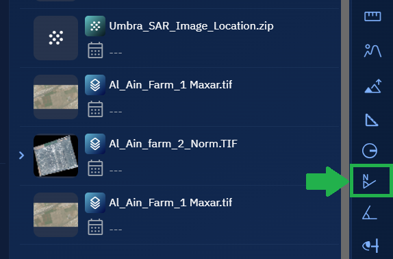
The Measurements dialog box is displayed.

2. Click on the map to set the starting point.

3. Click again to set the ending point.

   The system draws a line between the two points and calculates the bearing direction in degrees (°) from North.

4. Viewing the bearing result on the Measurements dialog box. The bearing angle will appear next to the measurement line.

Bearings are always measured clockwise from the geographic North.

Reviewing and Manage Bearing Measurements

After drawing a line, the Measurements dialog box will display the measured bearing — for example: 72.58°E.

If you draw multiple bearing measurements, each will be listed separately. For each entry, the following options are available:

Button	Description
Delete	Click to remove the corresponding line and its measurement from the map.
Copy	Click to copy the precise measurement value (e.g., 72.582994137) to a clipboard or notepad.

Measure Angle

The Measure Angle tool is used to determine the angle between two intersecting lines on the map. The angle is calculated in degrees (°) and displayed in the Measurements dialog box.

This tool is useful for analyzing spatial relationships and angular deviation between features such as roads, buildings, slopes, and more.

Prerequisites

• Open a layer with any source data

Use Cases

The Measure Angle tool is helpful in several geospatial analysis scenarios:

Use Case	Description
Infrastructure Planning	Measure angular deviation between roads, pipelines, or planned structures.
Urban Design	Analyze street intersections, building orientations, or zoning angles.

Using Measure Angle Tool

In this section, you will learn how to use the Measure Angle tool.

To use the Measure Angle tool, do the following:

1. Go to the Analyst Tools panel, and click the Measure Angle tool.

   

   The Measurements dialog box is displayed.

2. Locate a layer in which you want to measure angles.

3. Click on point A to set the starting point. Then click on point B to draw the first segment (line AB). Move the cursor to point C and double-click to complete the second segment (line BC). The system will calculate and display the angle formed at intersection point B between the two lines.

   

   The angle value is displayed on the screen.

4. Viewing the calculated angle in degrees (°) in the Measurements dialog box. Measurements are also displayed on the screen.

   The angle value is displayed next to the measurement line.

Reviewing and Manage Angle Measurements

After drawing an angle, the Measurements dialog box displays the measured angle — for example: 47.32°.

If you draw multiple angle measurements, each will be listed separately. For each entry, the following options are available:

Button	Description
Delete	Click to remove the corresponding angle and its measurement from the map.
Copy	Click to copy the precise angle value (e.g., 47.321834652) to a clipboard or notepad.

• Line of Sight Tool
  • Prerequisites
  • Use Cases
  • Getting Started with the Line of Sight Tool
  • Reviewing and Manage Line Measurements

Line of Sight Tool

The Line of Sight tool measures the straight, unobstructed distance between two points on a 3D surface. It helps determine whether there is a clear view (line of sight) between a starting location and a destination point, based on elevation data.

Prerequisites

Before you use the Line of Sight tool, ensure that a 3D Tiles layer with elevation data is loaded in your workspace.

• Open a workspace and load at least one 3D Tiles layer.
• To confirm the layer is loaded, check the Layers List panel. The 3D Tiles file should appear there.

important

If 3D Tiles layer is NOT loaded, the tool will still function but it will display a red line—even if there are no obstructions—because the elevation data needed for visibility analysis is missing.

Use Cases

The Line of Sight tool is valuable in a wide range of geospatial analysis scenarios where visibility between two locations is critical. Below are some common use cases:

Use Case	Description
Surveillance and Security Planning	Assess if observation towers or cameras have a direct line of sight to areas of interest.
Urban Development and Zoning	Evaluate how new structures (e.g., buildings, towers) may block views or interfere with sight lines.
Telecommunication Planning	Determine optimal placement of antennas or communication towers for unobstructed signal paths.
Emergency Response Planning	Ensure line-of-sight visibility between command centers and critical field locations.
Military or Tactical Analysis	Simulate lines of sight for strategic positioning, targeting, or defense planning.
Environmental Monitoring	Check if sensors or observation stations have visibility over target areas (e.g., forests, coastlines).

Using Line of Sight Tool

In this section, you will learn how to use the line of sight tool.

To use the line of sight tool, do this:

1. Go to the Analyst Tools panel, click Line of Sight tool.

   

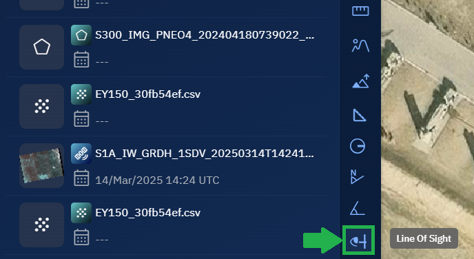
   The Measurements dialog box is displayed.

2. On the Measurements dialog box, click the Measure Units drop-down list to select one of the following units of measurement:

   • Meters
   • Kilometers
   • Feet
   • Miles
   • Nautical Miles

note

This unit determines how the distance will be displayed after the measurement is drawn.

3. Locate a layer with 3D tiles data in the Layers section, click the vertical three-dots menu, and then select the Zoom into Layer option.

   

4. Press and hold the Ctrl key and move your mouse up or down to tilt the map. Zoom in or out using the mouse scroll to view the 3D details on the map.

   Tilting the view helps you to visualize the 3D terrain and elevation details. This step is essential for using the Line of Sight tool effectively.

5. Click on the map to set the start point, draw the line, and double-click to set the end point.

   

   The system will now draw a line between the two points.

6. Viewing the measurement on the Measurements dialog box and interpret the result:

   • A green line indicates a clear line of sight — no obstructions between the points.
   • A red line means the view is blocked.

Reviewing and Manage Line Measurements

After drawing a line, the Line of Sight dialog box will display the measured distance next to the line — for example: 25.76 m.

If you draw multiple lines, each measurement will be listed separately.

For each entry, the following options are available:

Button	Description
Delete	Click to remove the corresponding line and its measurement from the map.
Copy	Click to copy the precise measurement value (e.g., 25.755476260316254) to a clipboard or notepad.

note

This tool allows you to easily manage, compare, or document multiple line of sight measurements as needed.